The Rocket’s Brain Pt. 2 — Target sighted!
A neural network controlled target-seeking rocket

In my previous article I built a neural network to control a target-seeking rocket in a two-dimensional space with pseudo-Newtonian physics. Because this had been my first attempt, I deliberately kept things very bare and simple: only the rocket existed in the simulation world, and furthermore its “sensors” always told it precisely where the target was. For this part I wanted to make the target a separate object in the world, and the rocket would need to locate it first before it could move towards it. Additionally there was now a rapidly dwindling fuel supply to take into account.
The new setup is not fundamentally different from part 1. The rocket’s physics are unchanged, including the sanity checks to ensure speed and rotation stay within reasonable limits. The main and rotational thruster systems are identical too, but are controlled slightly differently. I noticed in part 1 that the neural network outputs tended to have extremely large values which make them impractical to determine e.g. if we want only partial thrust. In effect, they were always full power or turned off, because the network could not evolve in such a way that smaller values showed up on the outputs. As a consequence I changed the interpretation of the network outputs to encode a 2-bit binary value for the thruster strength, with a threshold value that if exceeded encodes a binary 1, or a binary 0 if it is below. This means that there are four possible thrust levels: zero, one-third, two-thirds and full power. For the rotational thrusters I also needed a direction, so there is another binary output that encodes which direction the rotation fires. This gives five outputs total.
The network inputs were changed to reflect that the rocket doesn’t automatically know any more where the target is. In part 1 there were two inputs that directly fed the x- and y-position into the network. They were removed and replaced with six new inputs coming from each of the “radar sensors” that allow the rocket to see the target. They are arranged so that they cover 20° each of the full 120° field of vision to the front of the rocket. If the target is inside one of the sensor’s view it outputs a value proportional to the distance (the further away the target, the weaker). Five inputs for speed, direction and angular velocity were taken unchanged from part 1, and an additional one was added for the current fuel level (it wasn’t clear if this was strictly necessary or would have an effect). This gives a total of twelve inputs.
Early in the project I noticed that there were situations where the rocket would end up circling a target, but never quite get there, effectively “orbiting” it. I wondered if this was a fundamental problem of the setup because the neural net has no knowledge of the “history” so far, and as a possible remedy created a feedback input that connected to a looped back network output. I thought it might help trigger a break out of the stuck behavior. As it turned out this was unnecessary and there are working solutions where this input is unused (always is zero). I have left it in the source code but will ignore its existence in the following.
The network architecture was otherwise left unchanged and there were four layers, as in part 1.
The evolutionary algorithm was kept essentially unchanged, the population size was 1000 as in part 1 and used the same algorithms for mutation etc. The fitness computation was actually simplified: in every simulation step we add the distance to the target to the fitness score, and run the simulation until either the fuel runs out or the target is hit. If we don’t hit the target, double the accumulated fitness (making it a worse score since lower values are better).
The procedure for generalizing the solution was modified to work as follows:
- Start with one randomly generated “test case” (rocket starting point & target position).
- Run the population on the current set of test cases. If the best solution hits all the targets, or all targets but one, add two more random test cases for the next generation. This is as a compromise between having too many test cases to solve (costing too much computation time) and getting stronger feedback for the quality of the individuals.
- After each generation remove all test cases that were solved by at least half the population. This is to ensure that we don’t waste time solving too easy test cases that don’t provide enough of an incentive to improve. Top up the test cases to the previous full size with newly generated ones.
- Every 30 generations there is a “great filter” event where the number of test cases is increased to 100, or twice the last generation’s test cases, whichever is higher, for one generation, returning to the previous smaller size afterwards. This is another compromise to temporarily get higher precision for evaluating the quality of the individuals, in the hope that we weed out the overspecialized solutions and evolve towards a more general solution at lower cost than having a permanently high number of test cases.
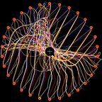
I arrived at this approach after some trial and error and found that the quality of the solutions improved rapidly. Unfortunately the computation times were noticeably higher than in part 1 too. The longest run took 14 hours and only reached 500 generations when I turned it off. In the end the solutions could successfully hit the target for over 250 test cases:

It resulted in a fairly effective solution (try it live here; press the “Randomize pos.” button to place the rocket in a random location and restart the simulation):
Thank you for reading!