The Rocket’s Brain

A personal project for tinkering with neural networks and evolutionary algorithms

• Read part 2 here
• Read part 3 here
• The JavaScript project on Github

Two ideas from computer science have intrigued me for a long time: neural networks and evolutionary algorithms. Neural networks are of course everywhere right now: essentially a computer runs a “brain” consisting of simulated nerve cells. They are being used to perform science-fiction-sounding tasks like besting human grand masters in games¹, creating natural looking landscapes from sketches² or even photos of people that don’t exist³. The concept behind evolutionary algorithms is possibly even more fascinating: a population of computer programs is tested against each other in a simulation of natural selection, and over time the descendants of the “survivors” become increasingly better at their required task. Although they are a bit less all-present than neural networks evolutionary algorithms have their applications, and sometimes both are used together.

Neural networks and evolutionary algorithms in their simplest forms can be programmed in surprisingly few lines of fairly straightforward code. Both are notorious for requiring a lot of computing power, but today’s computers should be plenty powerful enough to deal with a small problem even if the program runs in a web browser (or so I assumed). If I had an interesting problem to solve I could make an entertaining personal project that shouldn’t take lots of coding to complete, or so I hoped!

So I tried to come up with a very simple problem that’s also fun to look at. If it could become part of a video game, even better! The objective: hit a target (possibly an enemy UFO) with a homing rocket (possibly fired by the hero’s spaceship). It’s in “space”, a two-dimensional flat plane where the rocket is “fired” starting at some random position and the target is always at the origin of the coordinate system. The rocket can’t fly just any which way but rather experiences simulated (simplified) physics that allows believable (at least to me!) flying behavior. It needs a homing device that controls its main engine, which drives it forward, and two attitude jets on the sides that rotate it. Due to inertia the rocket will keep flying or rotating until the engines counteract that movement, so the homing device needs to take into account how the rocket is moving at all times to steer it successfully. This is definitely solvable in a variety of ways using handmade code, but I was curious how my neural network would handle it, if it could at all.

This project was made in JavaScript and runs on Firefox or Chrome browsers. You can find the source code here: https://github.com/rkibria/evolvenn

First I needed a working rocket simulation that was in a sweet spot of “complex enough” so that the rocket’s behavior is interesting but short of “needlessly complicated” which would increase the amount of code to write. The simulation’s complexity also affects how many inputs the neural network will have, unless we are willing to leave out some information, which I wanted to avoid.

The simulation uses 7 numbers (stored as 3 two-dimensional vectors and 1 number) to describe the rocket’s state:

• Position vector (where the rocket is). This changes according to the current velocity.
• Velocity vector (where the rocket is moving). This changes according to the current main engine’s thrust as well as the direction the rocket is facing.
• Direction vector (where the nose points). This changes depending on the current angular velocity.
• Angular velocity (turning speed). This changes depending on the attitude jets’ thrust.

These numbers will be fed to the neural network, which will compute from them how the engines fire. Two numbers control the engines:

• Acceleration (main engine thrust). If this is zero then the engine is idle, otherwise the velocity increases. Can only be positive.
• Rotation (attitude jet thrust). If this is zero then both jets are idle, otherwise one of the jets will thrust to turn the rocket clockwise or counter-clockwise.

As I found out later it was also necessary to introduce some sanity checks to avoid the rocket accelerating into infinity or turning so fast it looks like just a circle on the screen. Therefore the velocity as well as the angular velocity were locked to a maximum beyond which the engines will not push them.

The whole system is linked up like this:

When the program runs we read the current rocket state from the simulation at every time step and pass it through the neural network, which yields the rocket control values that we feed back to the simulation.

Now let’s build the actual neural network!

Neural networks are organized as layers of their basic elements, the neurons, which are very simplified models of nerve cells. Each neuron has a number of inputs and one output. The inputs are each associated with a constant number, the weights. The neuron sums up all inputs multiplied by the associated weight, and adds a flat bias value on top. Then the output of the neuron is the sum run through the neuron’s activation function: I used the rectifier⁴ which is equal to the sum if it’s larger than zero, or otherwise zero.

I am using a simple feedforward neural network setup where the inputs “ripple” through the layers starting from the inputs and come out the other end as outputs. The rocket simulation’s 7 output values will be the neural network’s inputs, and it should output 2 rocket control values to feed back to the simulation. However, as I found out from experimentation the rotation output presented a problem: as mentioned above it is supposed to be either negative to turn the rocket one way or positive to turn it the other way. This didn’t work very well and my rocket ended up only ever turning one way or not at all. Therefore I split up the rotation output into two outputs: one turns the rocket one way and the other the other way. Both are positive, but whichever is higher “wins” and turns the rocket its way, while the other output is ignored. So I ended up with 3 neural network outputs instead of 2, which have to be processed before passing the final 2 values to the simulation.

There was another range-related problem on the input side. The position input has a higher range of values than the others since it can reach e.g. high hundreds or more whereas the rest stay an order of magnitude or more lower. This seemed to hinder finding good solutions, so I added a logarithmic scaling to reduce the effective range of these two inputs.

This leaves the question of how many layers of neurons do I need? There is no precise answer to this⁵ and I arrived at using a total of 4 layers by trial and error. The first 3 layers (starting with the input layer) each have 7 neurons and the last layer (the output layer) has 3.

The complete neural network

Now the network’s high level architecture is decided it still needs to be able to solve the problem. This means the weight and bias values have to be assigned, of which there are rather many: in total we have 3 x (7 x 8) + 3 x 8 = 192 numbers to assign. Clearly too many to find by trial and error! This is where the evolutionary algorithm comes in.

At the heart of the evolutionary algorithm is a very simple loop:

1. Start with a population of solutions to our problem encoded in a way that supports mutating them.
2. Test every solution in the current population on a set of example problems. Assign each a fitness which is a number that measures how well the solution solves the problems.
3. Sort the solutions by fitness and “kill off” some percentage of the worst solutions. Fill the population up afterwards to the starting size with “offspring”, i.e. copies of the remaining solutions that have also been mutated. This is the next generation. Go to step 2 if the best solution found so far isn’t good enough, otherwise stop.

It’s expected that over time the population fills up with better and better solutions, hopefully including one that solves the problem at hand “well enough” so that we can stop. Since this is essentially a random search we can not guarantee to find an optimal solution and may need to run the algorithm many times.

The evolutionary algorithm

There are quite a few design decisions to make here. My implementation did the following, going for simplicity of implementation foremost:

• The solution encoding is a list of 192 floating point numbers (the neural network weights). Mutation means that I randomly vary each number in the list by a small amount up or down. The first generation starts with random numbers for every one of the list values.
• The population size is 1000 solutions.
• Step 3 always kills the worse half of the population. The “parents” are the other half, which create two offspring each, except the very best solution which is copied unchanged into the next generation.
• The mutation “rate” (how much an offspring will differ from the parent) changes over time. We have a high mutation strength at the start which halves every 100 generations. This was quite important for getting good solutions. The effect of this is that we try out very different solutions early on but concentrate on refining already good solutions later.

Assigning the fitness was not a straightforward endeavor and required quite a lot of trial and error until I got good solutions:

• Set initial fitness = 0. Set the initial rocket position somewhere not at the origin.
• Run the simulation for up to 10 seconds (effective time, not actual wall clock time). This equates to 600 simulation time steps, assuming 60 frames per second when running the graphical simulation.
• The rocket has hit the target if its position is within 20 units (half of drawn rocket length) to the origin. Stop the computation if hit but only if the rocket is hitting nose first. If not hitting nose first add 20 to the fitness and continue.
• If not hit, add the current distance to the origin minus 20 to the fitness score.
• After either 10 simulated seconds have passed or we hit the target multiply the fitness by 1 + steps taken / 60. If not hit in the 10 seconds double the fitness again.

The cumulative effect of these abstract rules is roughly “good solution get close to the center quickly and hit it nose first”. You may notice that the fitness value actually is higher for “bad” solutions: this is because traditionally evolutionary algorithms look for the lowest fitness value. This is a good fit here anyway but would be simple to fix if we wanted to look for the highest value instead.

Now both the neural network and the evolutionary algorithm are implemented, but how do we use this to find a solution that “always works”? Consider that in the description of the evolutionary algorithm we start the rocket at some (single) point, and generate a neural network weights set that can steer it from that point to the origin. What happens though if we don’t start at that exact point but somewhere slightly away from it, or even on the other side of the coordinate system? Unfortunately solutions that were generated for just one starting point do not work at all for anything else, the neural network is not general enough to “know what to do”.

How do we make it more general? Let’s assume a whole set of starting points and then running the fitness evaluation for each one, summing up the total fitness. If a solution has a good fitness for e.g. 100 starting points we could reasonably expect that the neural network has learned some general rules how to steer the rocket from anywhere rather than just “storing” a course that works for a single point. It’s not hard to make a loop over a large set of starting points like this, but this increases the computation times into unfeasible regions. Testing this approach with smaller sets of randomly placed starting points also showed that the resulting solutions were of poor quality, barely distinguishable from the single starting point solutions.

After more trial and error I found a compromise that worked:

1. Start with a single starting point, at a position just slightly below the origin.
2. Run the evolutionary algorithm until we have a solution that hits the target for every current starting point MINUS ONE. It was important not to require hitting for every starting point because sometimes the algorithm seemed not to find a way to make it happen and got stuck.
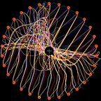
3. If we hit enough times, add an additional starting point. The new point is at the same position as the last one, but starts the rocket with the nose pointing in a different angle. Do this up to 4 times. After that, place the next point on a circle at the same radius as the last point. Repeat this until the circle is full, after that increase the radius by some amount and start with a point below the origin at this radius. ALSO every time we add a new point randomly vary the positions of every previous starting point by a small amount. This seemed to be important to make more general solutions.

This is the progress for a program run using this approach, sped up:

You can run the algorithm from this page: https://rkibria.github.io/evolvenn/evolve.html (warning, quite heavy on the browser!).

Since evolutionary algorithms are random searches that are likely to find some adequate solution but not always necessarily the optimal one it was not unexpected that many solutions were outright bad. Additionally there were also some that, though they do the job, were odd and not really “rocket-like” behavior:

• Early on, especially before I locked the maximum rotation speed down to a sane value, there were a lot of solutions that made the rocket spin like a Catherine wheel firework and fired the main engine only in the tiny moments it was pointed in a line to the center so that effectively the rocket had omnidirectional main thrust.
• After locking down the rotation speed there were a lot of solutions that still constantly spun and fired the main engine in a pattern that forward-then-sideways tumbled the rocket to the target a bit like a knight in chess.
• Some solutions looked mostly good except they would sometimes exhibit an odd “walking” behavior where the rocket would move almost straight sideways using only an attitude jet.
• When I tried to reward the algorithm for hitting the target with maximum speed and head on the rocket would always travel from wherever it started to some far point on one side of the target, then accelerate massively and hit from the same direction every time.

But eventually I got a solution that would hit the target fairly consistently starting from any point and looked reasonably realistic:

Try it out live on this page: https://rkibria.github.io/evolvenn/neural_sim.html (press the “Randomize pos.” button to place the rocket in a random location and restart the simulation).

Thank you for reading!

Click here to read The Rocket’s Brain Pt. 2: Target Sighted!

References

[1] https://deepmind.com/research/case-studies/alphago-the-story-so-far
[2] https://blogs.nvidia.com/blog/2019/03/18/gaugan-photorealistic-landscapes-nvidia-research/
[3] https://thispersondoesnotexist.com/
[4] https://en.wikipedia.org/wiki/Rectifier_(neural_networks)
[5] https://www.heatonresearch.com/2017/06/01/hidden-layers.html